Prerequisites - have Excel installed. That's it! Well, you'll also need the scorecard_template.xlsx and customers.xlsx files from here, and to put both of them in the C:\Users\Public folder on your machine. You may need to refresh the data source in scorecard_template.xlsx to populate the Data tab from customers.xlsx as well.
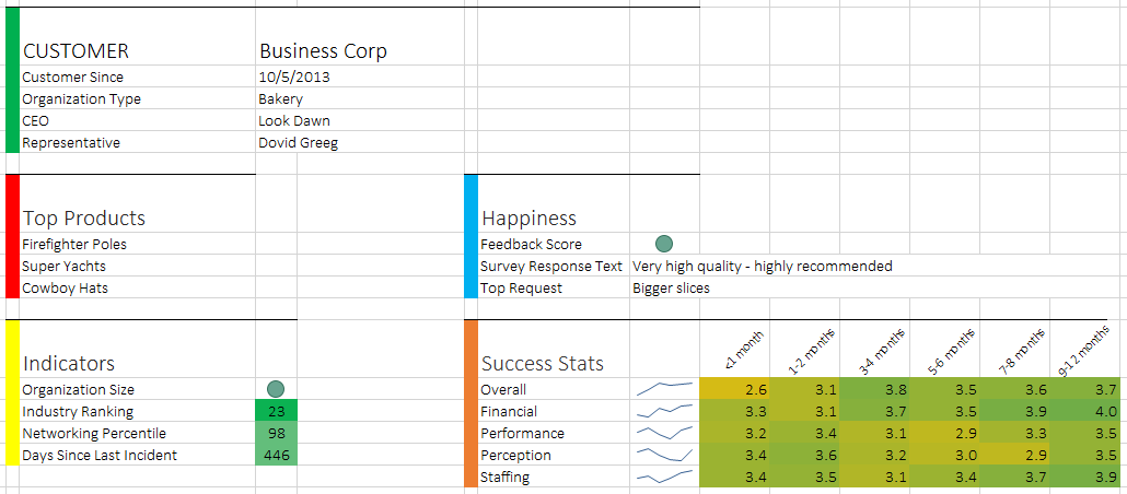
If you've ever wanted a quick & dirty way to visualize metrics & status info about something, there's a good chance you can get part of the way there without a fancy BI tool or a ton of time. Excel's visualization & conditional formatting tools, used in conjunction with references to data on another sheet, can easily product a scorecard like the one shown here:

We won't go through how to set up conditional formatting, sparklines, and drop-downs here. Take this as an FYI that these are possible in Excel, if you weren't aware - specific instructions are easy to find - I've included a few links to Microsoft's own resources below.
- Use sparklines to show data trends
- Use conditional formatting to highlight information
- Create a drop-down list
On the data tab we have a sheet of data called "Sheet1". As saved this may be empty - the source of the data is in customers.xlsx, to which we have a workbook connection which pulls the data. In other real life scenarios, connection may be to a SQL or Access database or something else. Hit "Refresh All" on the Data tab in Excel to query the data source and populate this tab with data. Doing so will cause the scorecard to populate.
Let's take a closer look at a formula field on the scorecard page. The feedback score field in row 9 / column 8 has the following formula
=INDEX(Sheet1[#All],MATCH(R2C4,Sheet1[Customer Name],0)+1,10)
We're using the INDEX function to look up a value in a data table. The table is provided by the first ("array") parameter, to which we've passed the value of "Sheet1[#All]" - our data sheet. This is where we'll use the customer selected from the drop-down to perform our lookup. The next parameter of the INDEX function takes a row number to use in our lookup - this will be the row number in our data table for our selected customer. We get this using the MATCH function - specifically we look to the selected customer from the drop-down (which lives in R2C4), and look up the row from the Customer Name column in Sheet1. The next parameter value of 0 simply means we're looking for an exact match, and we add 1 to the row number returned by the MATCH function because the first row in our table contains titles.
The final parameter value passed to INDEX - 10 - represents the column number of the data we want to pull from the data tab. Feedback score is stored in column 10, so that's what we put here. Most of the formulas on the scorecard sheet look just like this - only differing in which column of data they pull from the data tab.
The last thing we'll touch on is the Scoring Reference tab. Any cell that shows an icon or has a shaded color uses conditional formatting, as you can by selecting a cell and checking Home > Conditional Formatting > Manage Rules. You'll see that the thresholds which determine the color or icon of each cell are determined by the values on the Scoring Reference tab. This lets you see all thresholds in one place and edit them if you'd prefer different values.
And that's all there is to it! A handy dandy scorecard for entities of interest to you - easy peasy! In a subsequent post we'll discuss creating a Windows Forms application to do some of the reading and writing in C#, which will make things more interesting.
